Covariance-Matrix Notebook Workflow

Run the Published Package in Colab

The version-controlled Colab notebook is the simplest public reproduction path. It does not require a repository checkout. In a fresh Colab runtime it:

installs build-essential, libgsl-dev, and python3-dev;
installs the published wlcovpy==1.0.1 package from PyPI;
downloads Cls_ep2.txt and theta_array.txt from the matching v1.0.1 GitHub release tag;
carries its covariance helper functions directly in the notebook;
computes and validates the finite, symmetric 6 x 6 compact covariance matrix;
saves the numerical matrix and both diagnostic figures in the Colab working directory.

The version pin and tagged fixture URLs are intentional: they prevent a later package or input-file change from silently altering this documented result. The optional full R2D2 configuration is included but disabled by default because it performs many more native integrations.

Repository-Local Notebook

This page mirrors the structure of tests/notebooks/example.ipynb. The documentation is static, but the sections follow the same order as the notebook: setup, helper functions, input inspection, covariance calculation, plotting, and the larger R2D2 reference output.

The notebook uses the convenience functions in tests/python/covariance_example.py to wrap repeated wlcovpy calls in NumPy, then saves diagnostic plots in tests/notebooks/plots.

Unlike the self-contained Colab notebook, this development notebook imports the helper module and input files directly from the source checkout.

Open the interactive notebook from the repository root after building wlcovpy:

jupyter notebook tests/notebooks/example.ipynb

1. Setup

The first cell imports the scientific Python tools, finds the repository root, adds tests/python to sys.path, and creates the local plot directory.

from pathlib import Path
import os
import sys

import matplotlib.pyplot as plt
import numpy as np


def find_repo_root(start=Path.cwd()):
    for path in (start, *start.parents):
        if (path / "tests" / "python" / "covariance_example.py").exists():
            return path
    raise RuntimeError("Run this notebook from inside the 3ptWL-cov repository.")


REPO_ROOT = find_repo_root()
NOTEBOOK_DIR = REPO_ROOT / "tests" / "notebooks"
PLOTS_DIR = NOTEBOOK_DIR / "plots"
PLOTS_DIR.mkdir(parents=True, exist_ok=True)

sys.path.insert(0, str(REPO_ROOT / "tests" / "python"))
import covariance_example as cov

os.chdir(NOTEBOOK_DIR)

CLS_FILE = REPO_ROOT / "tests" / "input" / "Cls_ep2.txt"
THETA_FILE = REPO_ROOT / "tests" / "input" / "theta_array.txt"

print(f"Repository root: {REPO_ROOT}")
print(f"Plot directory:   {PLOTS_DIR}")

2. Helper Function Map

covariance_example.py keeps the notebook short by packaging the repeated steps:

add_noise_to_column writes a temporary noisy C_ell table;
build_mask selects the covariance entries to compute;
get_valid_indices converts that mask into index pairs;
calculate_integral runs one wlcovpy calculation;
compute_cov_noise assembles the symmetric covariance matrix.

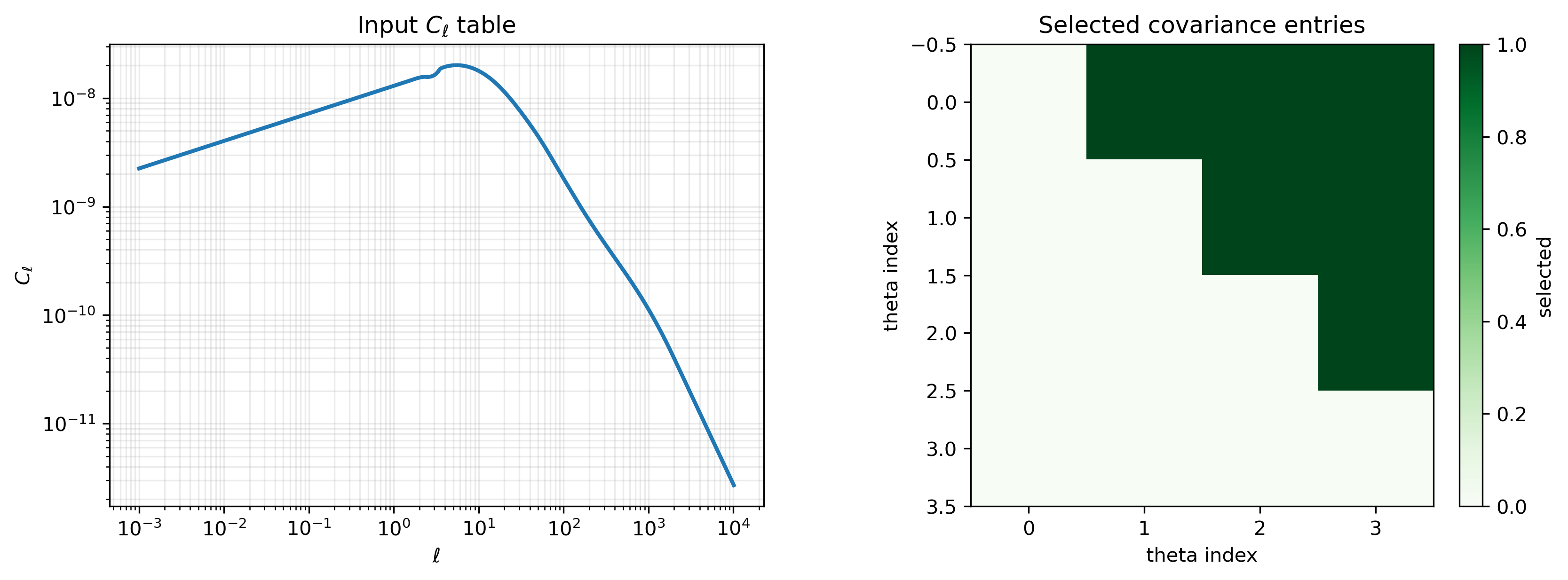
3. Inspect the Inputs

wlcov expects a two-column angular power-spectrum table, ell and C_ell. The covariance workflow also needs an angular grid. This compact example uses the first four angular values so it is fast enough for documentation and smoke tests.

ell, cls = np.loadtxt(CLS_FILE, unpack=True)
theta_all = np.loadtxt(THETA_FILE)

theta = theta_all[:4]
rows = 0
diagonals = 1
mask = cov.build_mask(dim=len(theta), rows=rows, diagonals=diagonals)

fig, axes = plt.subplots(1, 2, figsize=(11, 4), constrained_layout=True)

axes[0].loglog(ell, cls, color="#1f77b4", lw=2)
axes[0].set_title(r"Input $C_\ell$ table")
axes[0].set_xlabel(r"$\ell$")
axes[0].set_ylabel(r"$C_\ell$")
axes[0].grid(True, which="both", alpha=0.25)

im = axes[1].imshow(mask, cmap="Greens", interpolation="nearest")
axes[1].set_title("Selected covariance entries")
axes[1].set_xlabel("theta index")
axes[1].set_ylabel("theta index")
fig.colorbar(im, ax=axes[1], fraction=0.046, pad=0.04, label="selected")

fig.savefig(PLOTS_DIR / "inputs_and_mask.png", dpi=300, bbox_inches="tight")
plt.show()

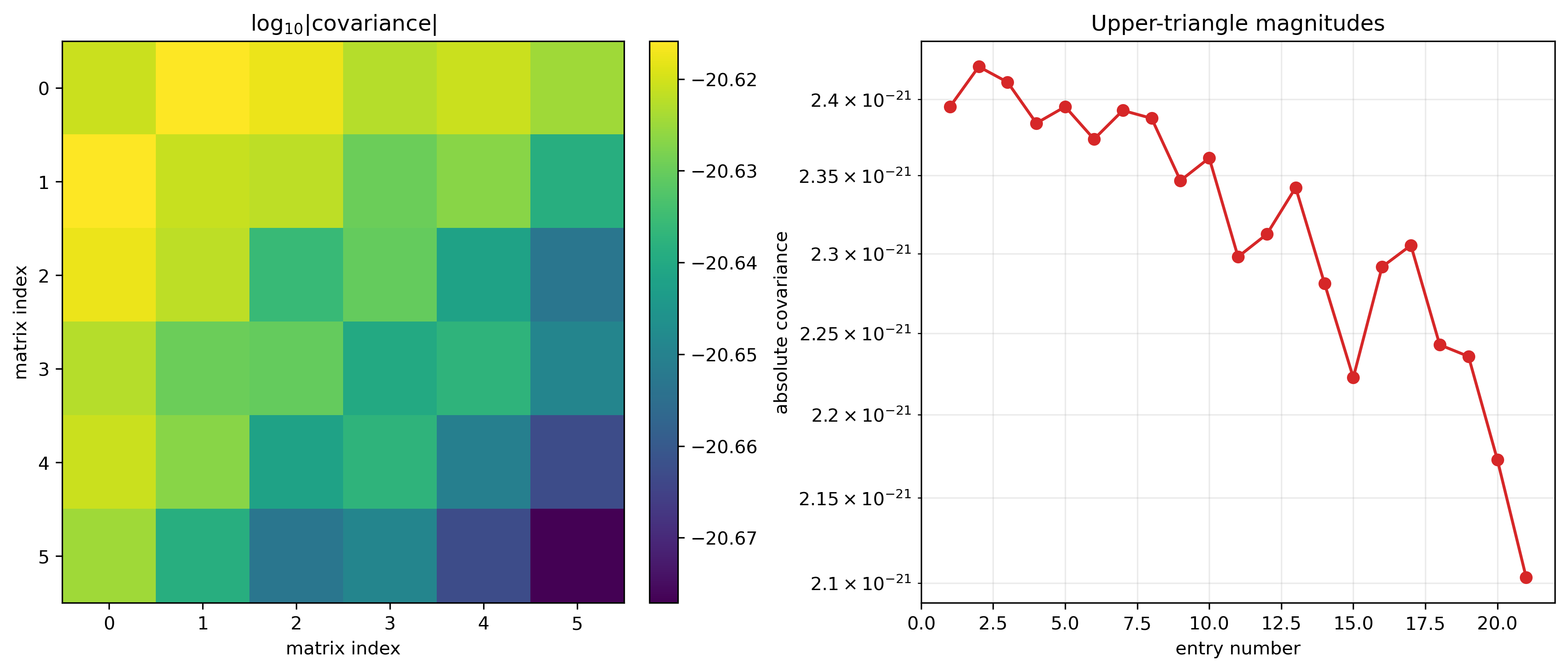
4. Compute a Compact Covariance Matrix

The helper adds a small noise term to the input spectrum, runs the covariance integral for each selected pair of angular scales, and stores the resulting matrix. The example uses a low ppp value because the goal is a quick documentation workflow, not a convergence-grade production run.

settings = dict(
    rows=rows,
    diagonals=diagonals,
    dim=len(theta),
    m=0,
    mp=0,
    ppp=4,
    noise=6.1e-11,
)

covariance = cov.compute_cov_noise(
    thtdata=theta,
    inputfile=CLS_FILE,
    outputfile=NOTEBOOK_DIR / "analytic_covariance_example.txt",
    **settings,
)

temp_file = NOTEBOOK_DIR / "Cls_temp.txt"
if temp_file.exists():
    temp_file.unlink()

print(f"Covariance shape: {covariance.shape}")
print(f"Finite values:    {np.isfinite(covariance).all()}")

The expected compact-example output is:

Covariance shape: (6, 6)
Finite values:    True

5. Plot and Save the Result

The main diagnostic plot is saved to tests/notebooks/plots/covariance_summary.png. The heat map shows log10(abs(covariance)); the right panel shows the magnitude of the upper-triangle entries.

abs_cov = np.abs(covariance)
log_cov = np.full_like(abs_cov, np.nan, dtype=float)
positive = abs_cov > 0
log_cov[positive] = np.log10(abs_cov[positive])

fig, axes = plt.subplots(1, 2, figsize=(12, 5), constrained_layout=True)

im = axes[0].imshow(log_cov, cmap="viridis", interpolation="nearest")
axes[0].set_title(r"$\log_{10}|\mathrm{covariance}|$")
axes[0].set_xlabel("matrix index")
axes[0].set_ylabel("matrix index")
fig.colorbar(im, ax=axes[0], fraction=0.046, pad=0.04)

upper_values = abs_cov[np.triu_indices_from(abs_cov)]
upper_values = upper_values[upper_values > 0]
axes[1].semilogy(
    np.arange(1, len(upper_values) + 1),
    upper_values,
    "o-",
    color="#d62728",
    lw=1.6,
)
axes[1].set_title("Upper-triangle magnitudes")
axes[1].set_xlabel("entry number")
axes[1].set_ylabel("absolute covariance")
axes[1].grid(True, which="both", alpha=0.25)

fig.savefig(PLOTS_DIR / "covariance_summary.png", dpi=300, bbox_inches="tight")
plt.show()

print(f"Saved: {(PLOTS_DIR / 'covariance_summary.png').relative_to(REPO_ROOT)}")

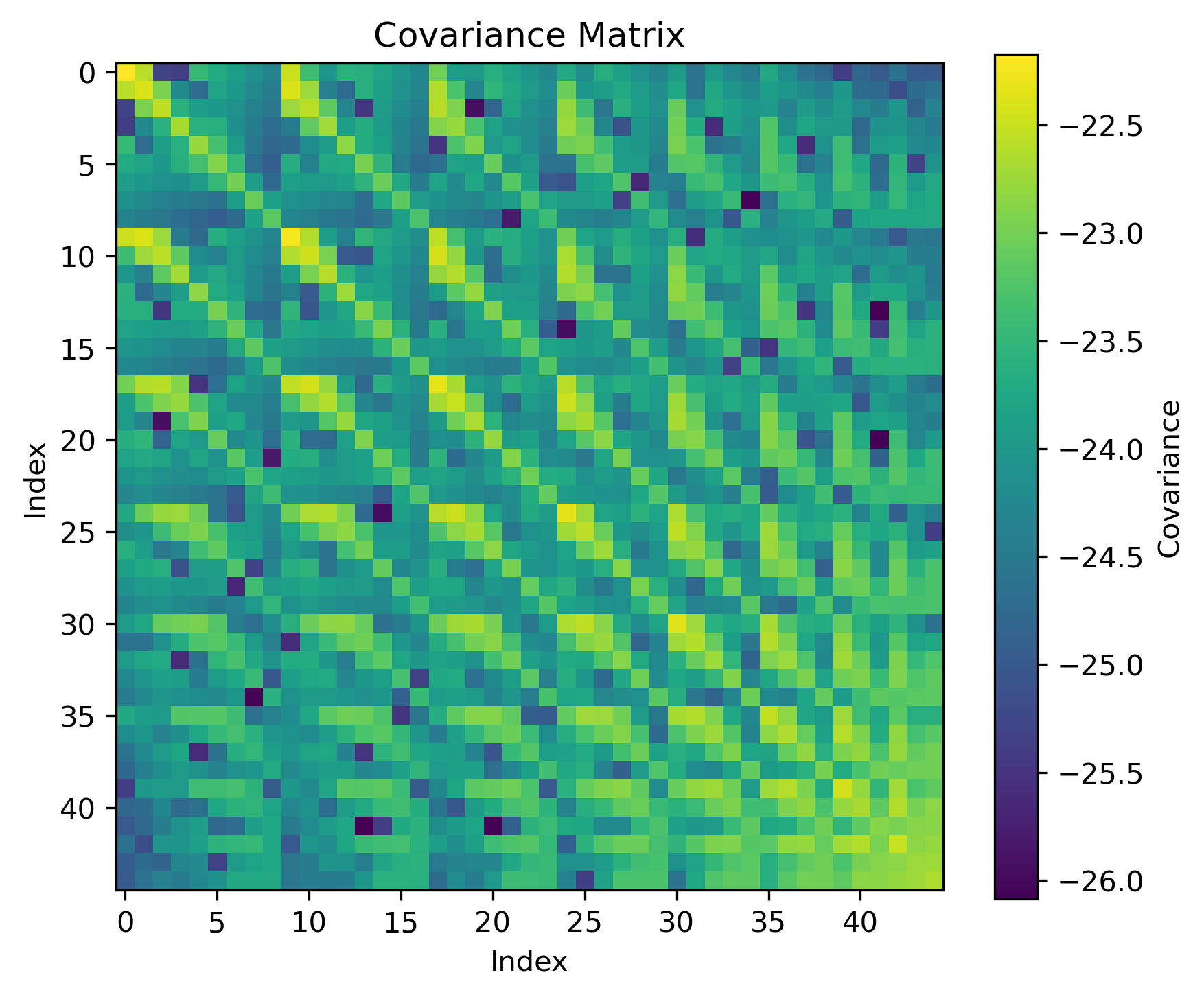
6. R2D2 Paper-Data Reproduction Workflow

The R2D2 workflow reproduces the covariance data used in the original paper. For this production-reference case, switch to the full theta array and use the larger mask parameters:

theta = theta_all
settings = dict(
    rows=7,
    diagonals=4,
    dim=20,
    m=2,
    mp=2,
    ppp=20,
    noise=6.1e-11,
)

The R2D2 reproduction workflow saves the reference covariance plot in tests/notebooks_r2d2/output_notebooks_r2d2/covariance_matrix.png:

Script Version

The notebook is based on tests/python/covariance_example.py. Run the script version from the tests directory when a command-line smoke test is more convenient:

cd tests
python3 python/covariance_example.py \
   --Cls-file input/Cls_ep2.txt \
   --theta-array input/theta_array.txt \
   --output analytic_covariance_quickstart.txt \
   --dim 20 --rows 7 --diagonals 4 --m 2 --mp 2 --ppp 20

The script:

creates a noisy temporary copy of input/Cls_ep2.txt;
builds a boolean mask over the requested covariance matrix entries;
calls wlcovpy.wlcov for each selected pair of angular scales;
writes the covariance matrix with numpy.savetxt;
writes a PDF heat map named analytic_covariance_22_noise.pdf.

For larger matrices, make the temporary C_ell filename and output directory unique for each process before parallelizing the workflow. The current example uses a shared Cls_temp.txt temporary file, so it should be run serially unless that filename is changed.